Creating a new workflow for oscillating data

In this tutorial we will consider a toy model to demonstrate how to extend the quickBayes package to solve new problems. At present all of the models must have the form:

\[y(x) = g(x) + \sum_{j=1}{N} f_j(x),\]

where \(g(x)\) is a function that is present in all of the models (e.g. background), \(f_j\) is the \(j^\mathrm{th}\) instance of the repeated function (e.g. sin) and \(N\) is the maximum number of repeated functions.

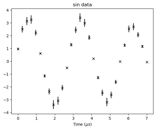
The first step is to read the test data and inspect it.

import matplotlib.pyplot as plt
import numpy as np

x, y, e = np.loadtxt('tutorial3.npy')

fig, ax = plt.subplots()
ax.set(xlabel='Time ($\mu s$)', ylabel='', title='sin data');
ax.errorbar(x, y, e, fmt='kx', label='data');

The quickBayes package does not currently have a sin fitting function as standard. Hence, we will create a new fitting function. Every fitting function must inherit the BaseFitFunction as this defines some useful methods that allow this class to be much simpler.

The __init__ has a super that take the number of arguments (3), the prefix, the starting guess as a list, the lower bounds as a list and the upper bounds as a list.

Next are the properties, these are used to create the text in the reporting. Each fitting parameter will need its own property. The inclusion of self._prefix allows for the full string to have some context, such as how many repeated functions are present.

The __call__ method is a simple evaluation of the fit function.

The read_from_report loads the results in from a report dictionary. This is done by repeating the _read_report for each parameter. The order of these must match those used in the report method. the report method adds the name and value for the fit parameter to the results dictionary.

from quickBayes.functions.base import BaseFitFunction
from numpy import ndarray
import numpy as np

class Sin(BaseFitFunction):
    def __init__(self, prefix=''):
        """
        :param prefix: prefix for function parameters in report
        """
        super().__init__(3, prefix, [1.75, 2.25, 0.22], [0., 0, 0], [5., 5., 2.])

    @property
    def amp(self):
        return str(f'{self._prefix} Amplitude')

    @property
    def freq(self):
        return str(f'{self._prefix} Frequency')

    @property
    def phase(self):
        return str(f'{self._prefix} phase')

    def __call__(self, x: ndarray, amp, omega, phi):
        return amp*np.sin(omega*x + phi)

    def read_from_report(self, report_dict,
                         index=0):
        """
        Read the parameters from the results dict
        :param report_dict: the dict of results
        :param index: the index to get results from
        :return the parameters
        """
        return [self._read_report(report_dict, self.amp, index),
                self._read_report(report_dict, self.freq, index),
                self._read_report(report_dict, self.phase, index)]

    def report(self, report_dict, amp, omega, phi):
        """
        reporting method
        :param report_dict: dict of parameters
        :param c: constant
        :return dict of parameters, including BG
        """
        report_dict = self._add_to_report(self.amp,
                                          amp, report_dict)
        report_dict = self._add_to_report(self.freq,
                                          omega, report_dict)
        report_dict = self._add_to_report(self.phase,
                                          phi, report_dict)
        return report_dict

The second thing that is needed to analyse the above data is a workflow. This will inherit the ModelSelectionWorkflow, which contains the common aspects of a model selection calculation. The preprocess_data method prepares the data for analysis, in this example it will just be a simple crop. The super sets the x, y, e values of the data we want to investigate.

The _update_function method defines what the workflow should do to add a repeated fitting function. Hence, it creates a Sin object and then adds it to the input function, which is then returned.

from quickBayes.utils.crop_data import crop
from quickBayes.workflow.model_selection.template import ModelSelectionWorkflow

class SinSelection(ModelSelectionWorkflow):

    def preprocess_data(self, x_data,
                        y_data, e_data,
                        start_x, end_x):
        """
        The preprocessing needed for the data.
        This crops and stores the data.
        :param x_data: the x data to fit to
        :param y_data: the y data to fit to
        :param e_data: the errors for the y data
        :param start_x: the start x value
        :param end_x: the end x value
        """
        sx, sy, se = crop(x_data, y_data, e_data,
                          start_x, end_x)
        super().preprocess_data(sx, sy, se)

    @staticmethod
    def _update_function(in_func: BaseFitFunction) -> BaseFitFunction:
        """
        This method adds a exponential decay to the fitting
        function.
        :param func: the fitting function that needs modifying
        :return the modified fitting function
        """

        function = Sin()
        in_func.add_function(function)
        return in_func

As with previous examples, we start by defining the parameters for the problem.

results = {}
results_errors = {}
start_x = 0.5
end_x = 6.3
max_features = 3

The next step is to setup the workflow, this will look almost identical to the other examples. This makes it easy to swap and change between different workflows.

workflow = SinSelection(results, results_errors)
workflow.preprocess_data(x, y, e, start_x, end_x)

In this case the unique functions are equal to zero. Therefore, we can just use an empty CompositeFunction.

from quickBayes.functions.composite import CompositeFunction

func = CompositeFunction()
workflow.set_scipy_engine(func.get_guess(), *func.get_bounds())
func = workflow.execute(max_features, func, func.get_guess())

Finally we get the loglikelihoods.

results, results_errors = workflow.get_parameters_and_errors

for key in results.keys():
    if 'log' in key:
        print(key, results[key][0])

N1:loglikelihood -12.365875723113799
N2:loglikelihood -11.631211270311063
N3:loglikelihood -937.4553937290698

To get the Bayesian P-value we first calculate the normalisation, by adding up the probabilities (note that the \(\log\) are base 10). Then we can report the P-values:

N = 0
for key in results.keys():
    if 'log' in key:
        N += 10**results[key][0]

for key in results.keys():
    if 'log' in key:
        print(f'P-value for {key.split(":")}', (10**results[key][0])/N)

P-value for ['N1', 'loglikelihood'] 0.15556193878162142
P-value for ['N2', 'loglikelihood'] 0.8444380612183786
P-value for ['N3', 'loglikelihood'] 0.0

It is clear that two sin waves are more likely for this example. However, one sin wave has a reasonable probability. We will plot the data along with the results for one and two sin waves.

fit_engine = workflow.fit_engine
x1, y1, e1, _, _ = fit_engine.get_fit_values(0)

fit_engine = workflow.fit_engine
x2, y2, e2, _, _ = fit_engine.get_fit_values(1)

fig, ax = plt.subplots()
ax.errorbar(x, y, e, fmt='ok', label='data')
ax.set(xlabel='time ($\mu s)$', ylabel='Asymmetry', title='input data');
ax.errorbar(x1, y1, e1, fmt='b--', label='1 sin wave')
ax.errorbar(x2, y2, e2, fmt='r--', label='2 sin wave')
ax.set(xlabel='Time ($\mu s$)', ylabel='', title='sin data');

plt.legend();

The plot shows that it is not unreasonable to have one sin wave, it does under and over estimate the values at the two extremes of the data. However, the two sin waves always has a good quality fit as expected.

The simulated data did use two sin waves. Hence, quickBayes was able to identify the correct model to use for this data.