QENS Example

This example is based on Quasi_Elastic Neutron Scattering (QENS) data as discussed by Sivia et al. It is used to examine a variety of molecular motions within a sample. For example, diffusion hopping, rotation modes of molecules and electronic transitions. This example uses real data collected at the ISIS neutron and muon source.

This example will demonstrate the QLData workflow for determining the number of Lorentzians in a sample. The first step is to import the correct packages. From quickBayes there are three imports;

• The workflow QLData

• The fitting function QlDataFunction

• A function for getting the background term from a string get_background_function

import os
import numpy as np
from quickBayes.workflow.model_selection.QlData import QLData
from quickBayes.functions.qldata_function import QlDataFunction
from quickBayes.utils.general import get_background_function

The data is contained within the test’s for quickBayes. Analysing QENS data requires both the sample measurements and the resolution. The resolution is used to reduce the background noise to zero, making it easier to identify the functional form of the data.

DATA_DIR = os.path.join('..', '..', '..', 'test', 'shared', 'data')

sample_file = os.path.join(DATA_DIR, 'sample_data_red.npy')
resolution_file = os.path.join(DATA_DIR, 'resolution_data_red.npy')

sx, sy, se = np.load(sample_file)
rx, ry, re = np.load(resolution_file)

resolution = {'x': rx, 'y': ry}

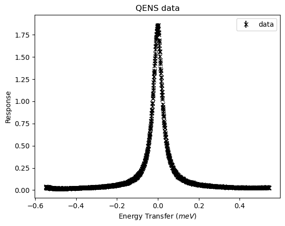
It would be helpful to have a look at the sample data. It shows a peak near to zero, which tapes off after about \(0.2\) (in either direction).

import matplotlib.pyplot as plt
fig, ax = plt.subplots()
ax.errorbar(sx, sy, se, fmt='kx', label='data');
ax.set(xlabel='Energy Transfer ($meV$)', ylabel='Response', title='QENS data');
plt.legend();

Matplotlib is building the font cache; this may take a moment.

The next step is to set the problem parameters. The results and results_errors are empty as we are doing a fresh calculation. The start value is chosen to be \(-0.4\) and the end value is \(0.4\), this is to make sure that there is some data that can be used for fitting the background values. The last value is the maximum number of Lorentzians to consider, in this case three.

results = {}
results_errors = {}
start_x = -0.4
end_x = 0.4
max_peaks = 3

The next step is to create a workflow object. This hides the complexity of the calculations and streamlines the code. For QENS data it is necessary to use preprocess_data, which interpolates the sample and resolution data onto the same x values. Hence, it returns the new x values and the corresponding resolution values (ry).

workflow = QLData(results, results_errors)
new_x, ry = workflow.preprocess_data(sx, sy, se, start_x, end_x, resolution)

QENS data can measure both the elastic and inelastic lines. We know that this data includes an elastic line, so it is set to true. This corresponds to a delta function in the fitting function.

elastic = True

The background is probably linear. The full fitting function is contained within QlDataFunction, which can hold an arbitrary number of Lorentzians. For N Lorentzians \(L\) with a background function \(BG(E)\) and an elastic line, the function is

\[y(E) = BG(E) + R(E)\circledast (A_0*\delta(E) + \sum_{j=1}^N L_j(E)),\]

where, \(E\) is the energy, \(R\) is the resolution function, and \(A_0\) is the amplitude of the delta function.

BG = get_background_function('linear')
function = QlDataFunction(BG, elastic, new_x, ry, start_x, end_x)

The function has some default bounds and starting guess. These are good enough for this tutorial. They are used to set the fitting engine in the workflow, at present there two available fitting engines are scipy and gofit (global optimization, see here for more details).

lower, upper = function.get_bounds()
guess = function.get_guess()
lower, upper = function.get_bounds()
workflow.set_scipy_engine(guess, lower, upper)

The workflow has an execute method, which does the required computations. This includes updating the fitting function to have the correct number of Lorentzians. It then returns the final fitting function, in this case a function containing three Lorentzians.

function_out = workflow.execute(max_peaks, function, guess)

The most likely function is the one with the largest logarithm of the posterior (loglikelihoods). This information is contained within the results dictionary, which can easily be accessed from the workflow. The following code will print out just the values for the loglikelihoods, where Nx indicates that it contains x Lorentzians.

results, results_errors = workflow.get_parameters_and_errors
for key in results.keys():
    if 'log' in key:
        print(key, results[key])

N1:loglikelihood [-659.4019084399863]
N2:loglikelihood [-349.1659820031302]
N3:loglikelihood [-350.8714576119793]

It is slightly more likely to have two Lorentzians than one. It could be helpful to visualise the fits from these calculations. The fit_engine contains the important information about the fits, including the results. The get_fit_values method takes an argument of the index of the fit (so in this case an index of 0 is one Lorentzian). It then returns:

• The x data

• The fitted y values

• The errors on the fit

• The difference between the fit and the original data (not interpolated)

• The errors on the differences

fit_engine = workflow.fit_engine

Lets look at each of the results one at a time, the range is reduced to give a better focus on the peak shape. First is a single Lorentzian.

x_data, y_data, e_data, df, de = fit_engine.get_fit_values(0)
fig, ax = plt.subplots()
ax.errorbar(sx, sy, se, fmt='k-', label='data')
plt.plot(x_data, y_data, label='fit 1 Lorentzian')
plt.plot(x_data, df, label='difference')
plt.legend()
ax.set(xlabel='Energy Transfer ($meV$)', ylabel='Response', title='QENS data');
ax.set_xlim([-.2, .2]);

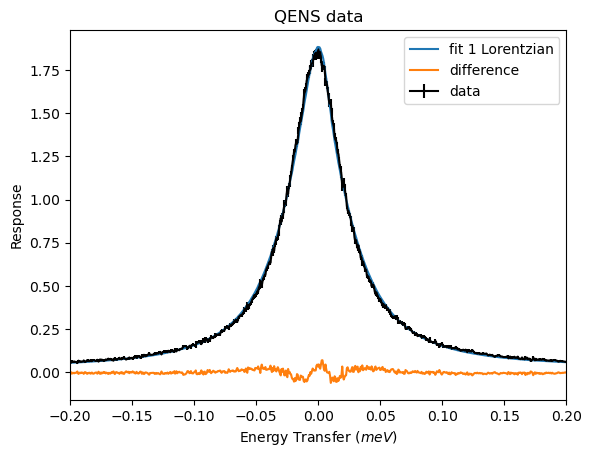
The fit appears to overestimate the top of the peak and underestimate just before the peak centre. This is further shown by the difference having a dip and then bump near to zero. This is not a very good fit, but it did have the worst loglikelihood value of -659.

x_data, y_data, e_data, df, de = fit_engine.get_fit_values(1)
fig, ax = plt.subplots()
ax.errorbar(sx, sy, se, fmt='k-', label='data')
plt.plot(x_data, y_data, label='fit fir 2 Lorentzians')
plt.plot(x_data, df, label='difference')
plt.legend()
ax.set(xlabel='Energy Transfer ($meV$)', ylabel='Response', title='QENS data');
ax.set_xlim([-.2, .2]);

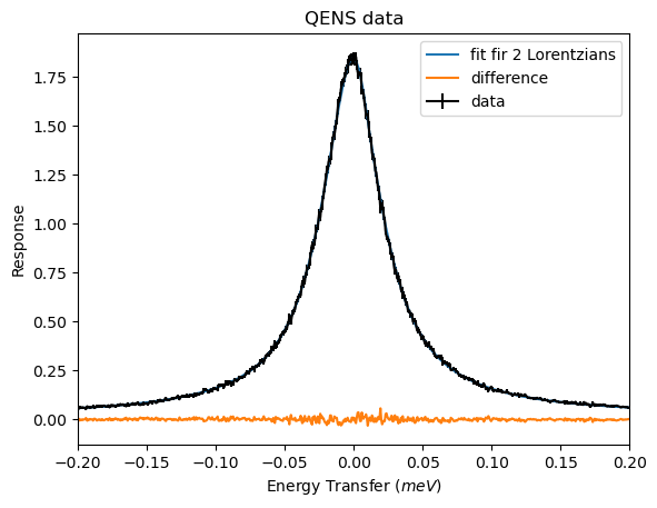
For two Lorentzians there does not seem to be any significant deviation between the data and the fit. This is expected as it had the best loglikelihood value.

x_data, y_data, e_data, df, de = fit_engine.get_fit_values(2)
fig, ax = plt.subplots()
ax.errorbar(sx, sy, se, fmt='k-', label='data')
plt.plot(x_data, y_data, label='fit')
plt.plot(x_data, df, label='difference')
plt.legend()
ax.set(xlabel='Energy Transfer ($meV$)', ylabel='Response', title='QENS data');
ax.set_xlim([-.2, .2]);

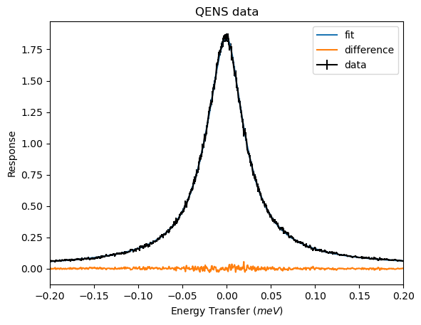
The three Lorentzians also produces a plot with no significant deviations. The logliklihood was only marginally worse than for two Lorentzians.

The last thing that might be of interest are the fit parameters and errors.

for key in results.keys():
    if 'N2' in key and 'log' not in key:
        print(key, results[key], results_errors[key])

N2:f1.BG gradient [0.0066597357953700155] [0.00030687459665655603]
N2:f1.BG constant [0.013764481830120434] [0.0002736238948039127]
N2:f2.f1.Amplitude [0.005037941758967548] [0.00034513237612374695]
N2:f2.f1.Centre [-0.0006646277296480829] [3.7087727664789324e-05]
N2:f2.f2.Amplitude [0.027228533382969305] [0.0012762619283654018]
N2:f2.f2.Peak Centre [-0.0006646277296480829] [3.7087727664789324e-05]
N2:f2.f2.Gamma [0.19554029117070532] [0.01025038342931913]
N2:f2.f3.Amplitude [0.13233755853763737] [0.00128014266839606]
N2:f2.f3.Peak Centre [-0.0006646277296480829] [3.7087727664789324e-05]
N2:f2.f3.Gamma [0.043860767406203115] [0.0005897110674049834]
N2:f2.f2.EISF [0.156135485416556] [0.0242207487938627]
N2:f2.f3.EISF [0.036672781886800926] [0.010936770134154075]