Muon Decay Rates

In this example we will look at some simulated muon spectroscopy data. This data has been used at the ISIS Neutron and Muon source to test software. The simulated data is described by a background plus some exponential decays. The decay constants can indicate the muon stopping site or the relaxation time for the muon, depending on the experimental setup. There can be multiple muon stopping sites or relaxation times within a sample, so it is important to be able to identify the number of exponential decays.

The first step in the analysis is to import all functionality that we will need. From quickBayes there are three imports;

• The workflow MuonExpDecay

• A function for adding fitting functions CompositeFunction

• A function for getting the background term from a string get_background_function

from quickBayes.functions.composite import CompositeFunction
from quickBayes.utils.general import get_background_function
from quickBayes.workflow.model_selection.muon_decay import MuonExpDecay
import numpy as np
import matplotlib.pyplot as plt
import os

The data is contained as part of the tests for quickBayes. On loading the data it can be useful to visually inspect it.

DATA_DIR = os.path.join('..', '..', '..', 'test', 'shared', 'data', 'muon')
data_file = os.path.join(DATA_DIR, 'muon_expdecay_2.npy')

sx, sy, se = np.loadtxt(data_file)

fig, ax = plt.subplots()
ax.errorbar(sx, sy, se, fmt='kx', label='data');
ax.set(xlabel='Time ($\mu s$)', ylabel='Asymmetry', title='Muon data');
plt.legend();

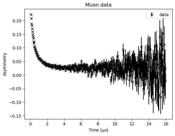
Looking at the data its not obvious how many decays are present (the name of the file tells us that the answer is two). To continue we need to set the problem definition. The start value is set by the time zero of the experiment and the end point is chosen based on the signal to noise ratio. The maximum number of decays that we want to consider is three. The results and results_errors are empty as we are doing a fresh calculation.

start_x = 0.16
end_x = 15.0
max_features = 3
results = {}
results_errors = {}

The workflow contains most of the complicated calculations. The workflow takes the results and results_errors and will append to them. The next step is to prepare that data for analysis using the preprocess_data method, in this case it just crops the data between the start and end values.

workflow = MuonExpDecay(results, results_errors)
workflow.preprocess_data(sx, sy, se, start_x, end_x)

The function we want to consider is a function of time (\(t\)) of the form

\[y_N(t) = ct + \sum_{j=1}^{N} A_j \exp(-\lambda_j t),\]

where \(c\) is a constant background value, \(A_j\) is the amplitude of the \(j^\mathrm{th}\) decay, \(N\) is the number of decays being considered and \(\lambda_j\) is the decay rate of the \(j^\mathrm{th}\) decay.

First we use the get_backgound_function to get a constant background (flat), the other options are None and linear. The CompositeFunction is a wrapper for adding fitting functions together, this is done by using the add_function method.

BG = get_background_function('flat')
func = CompositeFunction()
func.add_function(BG)

It is helpful to know the default bounds for the fitting function, this can be obtained with the get_bounds method.

lower, upper = func.get_bounds()
print('lower bounds', lower)
print('upper bounds', upper)

lower bounds [-1.0]
upper bounds [1.0]

Looking at the plot above, it is clear that these bounds are too large. We can set them using the set_bounds method, it takes a list of the lower and upper bounds as arguments. The final optional argument is the index this tells the CompositeFunction which function the new bounds should be associated with, by default it is the last function to be added to the CompositeFunction.

func.set_bounds([-.1], [.25])
print(func.get_bounds())

([-0.1], [0.25])

There is also a get_guess method for getting the start values for a fit. If these are not suitable then it can be updated using the set_guess method. The arguments are the new guess and the index of the function you would like to update (the default is the last function to be added).

print(func.get_guess())

[0.0]

The workflow requires a fitting engine to compute the results. At present there are two options scipy and gofit (global optimization, see here for more details). The next line executes the workflow, this will calculate the log of the posterior probability for one to four decays, along with the corresponding fitting results. It returns the last fitting function it used, in this case four decays plus a flat background.

workflow.set_scipy_engine(func.get_guess(), *func.get_bounds())
func = workflow.execute(max_features, func, func.get_guess())

The results and errors of the calculation can be obtained from the get_parameters_and_errors method. This returns two dictionaries, one for the values and one for the errors. The keys indicate the parameter, with the Nx showing how many features (decays) were used in the calculation. Within the results are the loglikelihoods (\(log_{10}(P)\)), which are the logs of the unnormalized posterior probability. Hence, the most likely model is the one with the largest value. When the loglikelihood is calculated it does not take the background into account (other than being part of the \(\chi^2\) value). Since the background is the same function in all of the models it just adds an offset to the loglikelihood, so it is neglected.

results, results_errors = workflow.get_parameters_and_errors
for key in results.keys():
    if 'log' in key:
        print(key, results[key][0])

N1:loglikelihood -161.625454386235
N2:loglikelihood -113.54837843974272
N3:loglikelihood -372.3725153229217

The results show that two decays are most likely, followed by one decay. The code includes a penalty for overfitting, this reduces the probability of a model that is overparameterized.

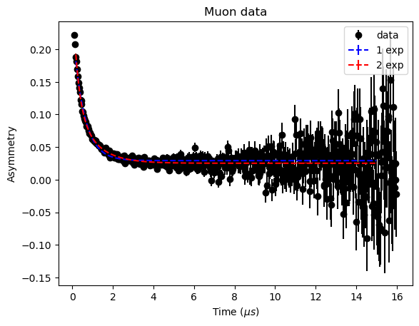
It would be helpful to view the fits against the data. To do this we get the fit_engine object directly, which keeps a history of the fits it has performed. The fit_engine has a get_fit_values method that returns;

• the x data

• the fitted y values

• the errors on the fit

• the difference between the fit and the original data (not interpolated)

• the errors on the differences

for the requested fit. The first fit was for one decay, so will be at index 0.

fit_engine = workflow.fit_engine
x1, y1, e1, _, _ = fit_engine.get_fit_values(0)

fit_engine = workflow.fit_engine
x2, y2, e2, _, _ = fit_engine.get_fit_values(1)

Plotting the results with the data shows how difficult it is to determine the number of decays by eye. The simulation was for two decays, so the workflow has correctly identified the number of decays.

fig, ax = plt.subplots()
ax.errorbar(sx, sy, se, fmt='ok', label='data')
ax.set(xlabel='time ($\mu s)$', ylabel='Asymmetry', title='input data');
ax.errorbar(x1, y1, e1, fmt='b--', label='1 exp')
ax.errorbar(x2, y2, e2, fmt='r--', label='2 exp')
ax.set(xlabel='Time ($\mu s$)', ylabel='Asymmetry', title='Muon data');

plt.legend();

The fit parameters for the two decays are contained within the results dictionary and the results_errors has the corresponding errors. It is important to note that the loglikelihoods do not have corresponding error measurements.

for key in results.keys():
    if 'N2' in key and 'log' not in key:
        print(key, results[key][0], results_errors[key][0])

N2:f1.BG constant 0.025188493466352085 0.0005977810369605421
N2:f2.Amplitude 0.16777171881687614 0.008152472164156299
N2:f2.lambda 3.8643084042142055 0.34286694511857513
N2:f3.Amplitude 0.09672961818656674 0.011012092991570709
N2:f3.lambda 1.0149730115894025 0.08170507981548476